Adversarial Search (Chapter 5)
Zero-sum
Initially we focus on games that are deterministic and completely observable. We also assume that the payoff to each player at the end of a game is equal and opposite, called zero-sum. To get a true sum of zero, some games require subtraction from each outcome. Imagine a win is value 1, a loss is value 0, and a draw is 1/2.
| Result | Subtract 1/2 | |
|---|---|---|
| Win,Loss | Player A = 1, Player B = 0 | Player A = 1/2 Player B = -1/2 |
| Draw | Player A = 1/2, Player B = 1/2 | Player A = 0, Player B = 0 |
Definition of a game:
- initial state $s_0$
- $player(s)$: which player is to move in state $s$,
- $actions(s)$: legal actions from state $s$,
- $result(s,a)$: state that results, like our
take_action_f - $terminaltest(s)$: true when game is over
- $utility(s,p)$: payoff for player $p$ upon reaching state $s$.
Minimax
The two players in a two person game will be called Max and
Min. These names reflect the meaning of the $utility(s,p)$
function, which is to be maximized by Player Max and minimized by
Player Min.
The partial search tree in this next presentation illustrates the reasoning behind the concept of alternate layers minimizing and maximizing the utility value to back up a value from terminal states to non-terminal states.
from IPython.display import IFrame
IFrame("http://www.cs.colostate.edu/~anderson/cs440/notebooks/minmax.pdf", width=800, height=600)
The calculation of the minimax(s) value of a state $s$ can be
summarized as
Assumes player Min plays optimally. If not, Max will do even
better.
The textbook shows in Figure 5.3 the minimax-decision algorithm as
a depth-first search that altenates between calling max-value and
min-value functions.
Alpha Beta Pruning
Some of the search tree can be ignored if we know we cannot find a better move from the best one found so far. If you are Player X in Tic-Tac-Toe, and
- your best move so far will result in a draw, and
- the next move you are evaluating you discover your opponent can definitely win from,
- do not explore any other choices your opponent might have.
IFrame("http://www.cs.colostate.edu/~anderson/cs440/notebooks/alphabeta.pdf", width=800, height=600)
For each node, keep track of
$alpha$ is best value by any means
- Any value less than this is no use because we already now how to achieve at least a value of $alpha$
- Minimum value Max can get
- Initially, negative infinity
beta is worst value for the opponent
- Anything higher than this won't be useful to opponent
- Maximum score Min can get
- Initially, infinity
The span between alpha and beta progressively gets smaller.
Any position for which beta < alpha can be pruned.
IFrame("http://www.cs.colostate.edu/~anderson/cs440/notebooks/alphabetatictactoe.pdf", width=800, height=600)
Stochastic Games
First, a definition of expected value. The average value of a lot (infinite number) of dice rolls with a fair dice is
$$ (1+2+3+4+5+6) / 6 $$The expected value is exactly this average, but is defined as the sum of the possible values times their probability of occurring.
$$ 1(1/6) + 2(1/6) + 3(1/6) + 4(1/6) + 5(1/6) + 6(1/6) $$If the 4, 5 and 6 sides are less likely than the other sides, then the expected value might be
$$ 1(1/4) + 2(1/4) + 3(1/4) + 4(1/12) + 5(1/12) + 6(1/12) $$A stochastic game is modeled by simply adding a level of chance nodes between each player's levels in the search tree. The various outcomes from the chance node have certain probabilities of occurring. When backing up values through a chance node, the values are multiplied by their probability of occurring.
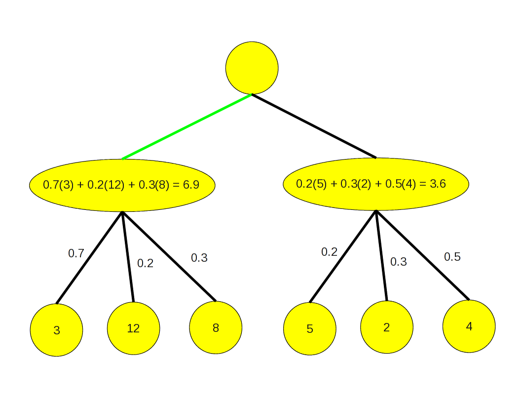
This illustrates the expectimax algorithm, for backing up values through chance nodes.
An alternative approach is to do Monte Carlo simulation to estimate the expected values. Perform many searches from the same node and at each chance node select just one outcome with the corresponding probability. Average over the resulting backed up values. Sometimes called a rollout.
Can alpha-beta pruning be applied to the expectimax algorithm?
Seems like the answer is no; we must know all children to calculate their weighted average values. But bounds can be placed on the possible average value if we know bounds on the utility values.
Can evaluation functions be applied to non-terminal nodes in stochastic games? Yes, but must be careful, as Figure 5.12 illustrates. Evaluation functions must be a positive linear transformation of the expected utility from a position.